ArrayPipe Online Documentation

Estimating the predictive power to be gained from an experiment

This section helps to figure out the answer to two common questions that often come up when dealing with microarrays:

How many replicates do I need?
Which fold-changes can I trust?

The first one should be asked when designing the experiment and the second one is of interest when the slides are being analyzed. In both cases the answer depends strongly on the amount of data variation that exists between replicates.

ArrayPipe provides a solution for the calculation of data variation that is closely modeled after a method described by Wei, Li, and Bumgarner (2004) Sample size for detecting differentially expressed genes in microarray experiments. BMC Genomics 5:87.

The main idea behind this is to calculate for each spot on the array the standard deviation between the log2 ratios of the replicates on which a statistical test is supposed to be carried out. These values are ranked in increasing order and the user can choose a cut-off, which they feel comfortable with. The acquired value is then inserted into a standard formula for power calculation, which generates the number of samples needed or the fold-change that is detectable under certain conditions (more details below).

The next graphic shows how the module 'Calculation of variation' (section 5, 'replicate handling') is applied (click on image for a larger version):

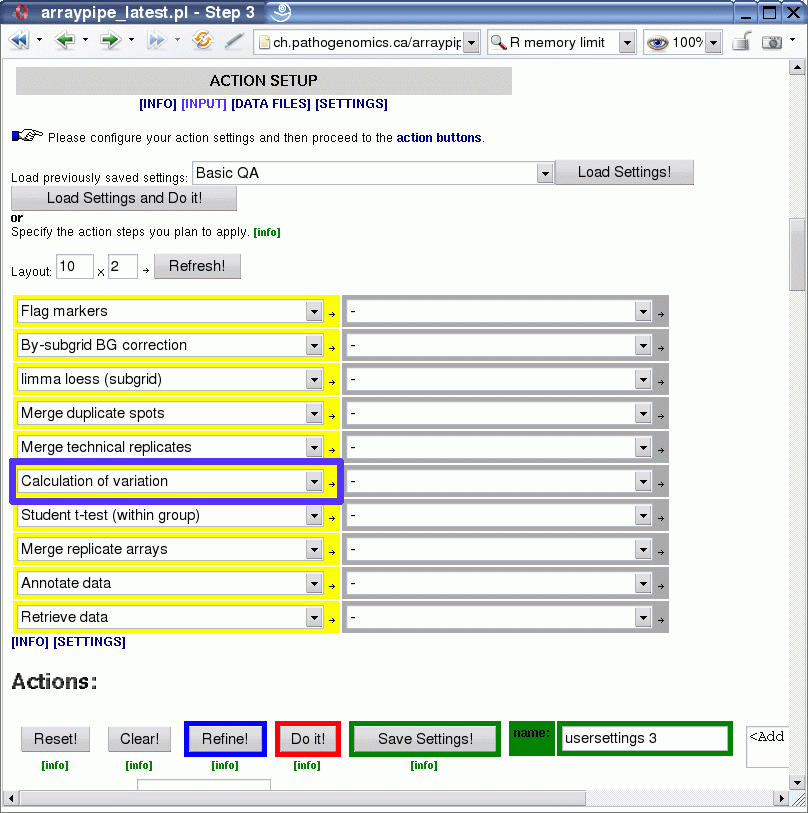
Some standard analysis steps are applied to a set of slides:

flagging of markers
background correction
print-tip normalization with loess
merging of duplicate spots
merging of technical replicates

Let the experiment describe three different conditions (treatments or time-points), and for each condition, 6 slides are available, which represent 3 biological replicates with two technical replicates each. After the above steps we would now have three sets of merged slides for each condition.

This is the point were normally something like a one-sample t-test is carried out to detect for each condition, which genes show expression changes that are significantly different from 0 (on the log-2 scale). Therefore, we will insert the variation calculation here, to let it work on the same input, i.e. it will calculate the variation between the three biological replicates in each treatment group.

The output looks something like the following:

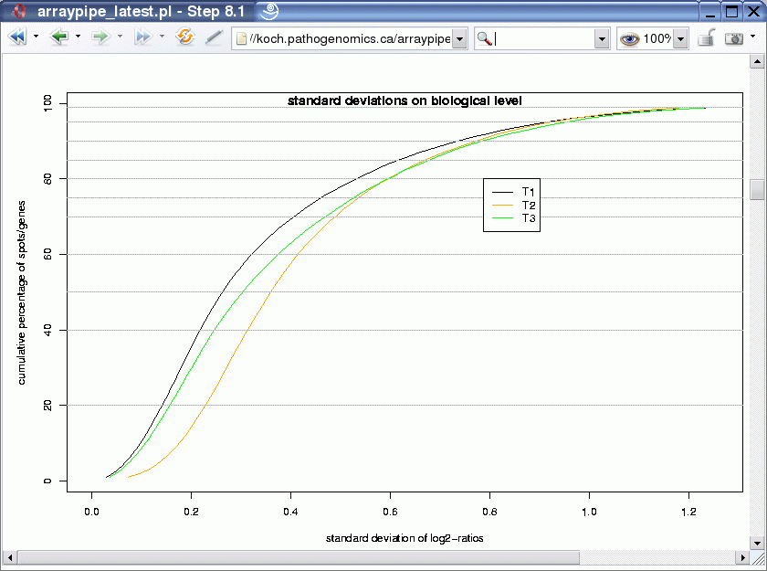
The graph shows three curves, one for each treatment. It plots the variance representative for a certain percentile in the ordered list of standard variations. For example, the standard variation for the least 80% variable genes reaches nearly 0.6 for treatments T2 and T3, whereas it is a little bit lower for treatment T1.

For some selected percentages, the variations are presented in a table:

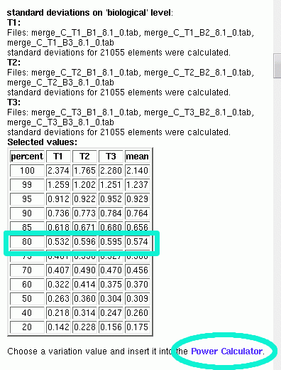
From that you can read out the exact values for each treatment group and also get the average. It is up to the user to define a threshold which determines the value of data variation used for the power calculation.

Following the link circled in the above image one gets to the Power Calculator, a web front-end to the power.t.test function in R. It allows you to

compute the power of a test, or
determine parameters to obtain target power.

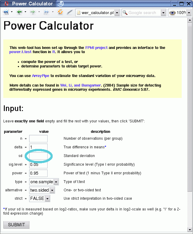
Insert the variation value (chosen from the table or the graphic in the ArrayPipe output) into the field for standard deviation (sd) circled below:

After clicking on the submit button you receive the output, which consists of the value for the one variable that was left empty, in this case the number of replicates:

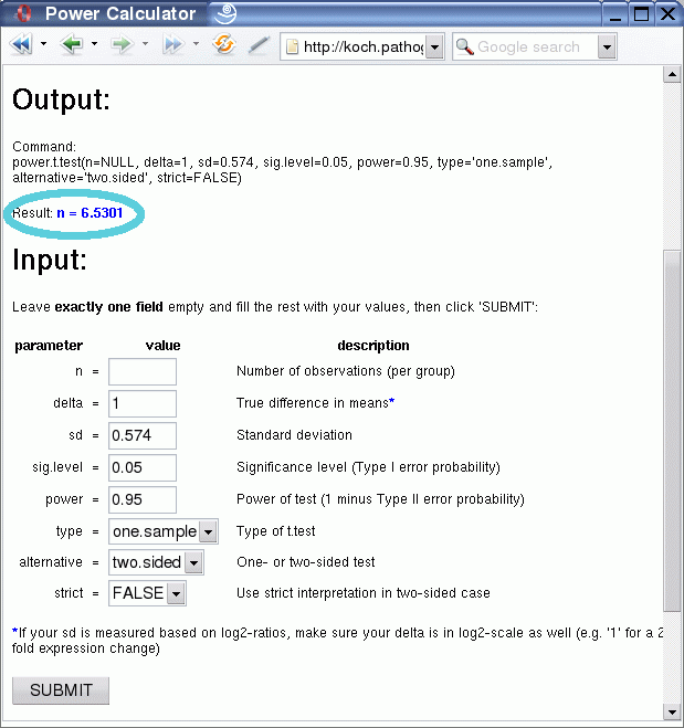
The result shows that at least seven biological replicates would be necessary to reliably detect 2-fold expression changes (1 on log2-scale!) with 95% power at 0.05 significance level for the given variation, using a two-sided one-sample t-test.

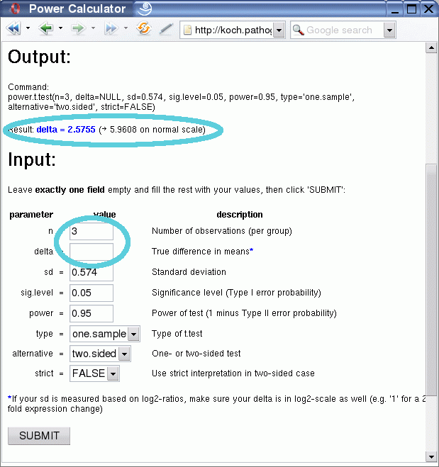
One might ask now, what level of expression change can be detected with the given number of replicates that are available? This can be easily answered, by changing the value for n to 3 and deleting the entry for delta.
After clicking the submit button you will be presented with the result: 2.58 on log2-scale or 5.96 on the normal scale (fold-changes).

Please keep in mind that this method leaves a lot of space for parameter modifications, depending on the users preferences. For example, do you require a 95% power level or a 0.05 significance level? This depends on how much of Type I and Type II error you are willing to tolerate. Also, the percentage of data from where you choose the variation level is up to you. The procedure described above provides simply some guidelines to give an indication of the power that can be gained from a microarray experiment.

In addition to the power calculation, the ArrayPipe module for the calculation of variation can be used to quickly determine flawed slides. For example, carrying out the function at an early stage, before the technical replicates are merged, generates the following output:

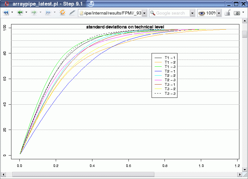
For each biological replicate in each treatment group we can find the variation amongst the two technical replicates. If one of the slides were flawed it would result in a curve at higher levels of standard deviation, which would stand out from the rest. In this case the technical replicates for biological sample 2 in treatment T2 (dark blue curve) seems to perform a little bit worse than the other sets and might require closer investigation.

[← previous] [up ↑] [next →]

Home

last modified $Date: 2007/08/27 14:02:03 $
for questions or remarks e-mail karsten_hokamp@sfu.ca.