Cerebral Tutorials
In this set of tutorials, you will install the Cerebral Cytoscape plugin, learn how to create and interact with a Cerebral layout, and learn how to use the features of Cerebral v.2's multi-experiment comparison tool. A sample dataset will be used throughout - this is a small representation of the TLR4 signalling pathway, an important immune pathway involved in the response to Gram-negative bacteria. The dataset is derived from a 2006 paper from our group (Mookherjee et al., Modulation of the TLR-mediated inflammatory response by the endogenous human host defense peptide LL-37, J. Imm. 176(4):2455-64), reporting the results of a two treatment/four timepoint microarray experiment. This file contains a subset of the data - two treatments (LPS alone, LPS+LL-37) at one timepoint (4h). The fold changes provided in the sample file are real, however the p-values have all been set to 0.01.
- Tutorial Part 1: Creating a Cerebral view
- Tutorial Part 2: Interacting with a Cerebral view
- Tutorial Part 3: Using the multi-experiment viewer tools
Tutorial 1: Creating a Cerebral view
Step 0: Installing the Cerebral plugin This step only needs to be performed once.
0.1: Download both the latest version of cerebral.jar and prefuse.jar from the Cerebral Downloads page.
0.2: Save the two files in Cytoscape's plugins directory.
0.3: Launch Cytoscape and ensure that the plugins are loaded - if successful, you will see the Cerebral tab in Cytoscape's Control Panel. In the Plugins menu you will see Create Cerebral view, Restore previous Cerebral views and Export Cerebral view. These may take a few seconds to appear after Cytoscape opens.
Step 1: Loading the sample data
1.1: Download the XGMML file containing all necessary data for the TLR4 network and experiment: tlr4_tutorial.xgmml (right-click and Save As).
A word about the information you need to run Cerebral: In order to generate a localization-based layout, Cerebral requires you to provide localization annotation for as many of the nodes in your network as possible. There are many sources for such data (see our Links page for a list), however once you have collected the information, it must be stored in a format that Cytoscape is able to read in. This can be as a node attribute or spreadsheet file. The text values for the localization attribute can be whatever the user desires - Cerebral will read in any text - but please note that the values are case-sensitive, so "cytoplasm" and "Cytoplasm" will be treated as two separate localization sites by the algorithm.
1.2: Load the data by selecting File > Import > Network (multiple file types) from the Cytoscape menu or using the Ctrl-L keyboard shortcut. The network will appear in the main Cytoscape panel. Node labels may be missing - to turn them on, select "ID" as the target of the passthrough mapper in Cytoscape's VizMapper then click in the network to make them appear. For more assistance on the VizMapper, view the Cytoscape manual VizMapper page here.
1.3: To see the attribute data contained in the TLR4 sample file, click the "Select Attributes" icon in Cytoscape's Data Panel and place checkmarks next to the Localization, Function, and LPS/LPS+LL-37 attributes. Selecting a node or nodes will make their attribute values visible in the Data Panel.
Step 2: Performing the layout
 2.1: From the Plugins menu, select Create Cerebral view
2.2: Select the attribute containing the localization information from the first dropdown menu. In our tutorial this is the Localization attribute.
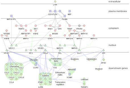
2.3: The attribute values in the loaded file will be used to populate the layer placement table. Cerebral divides the Cytoscape window into horizontal stripes, one for each localization site read in from the attribute file. By highlighting a row and using the arrow buttons to move the row up or down, you can control the order that these stripes will be arranged in. We recommend ordering that provides a cross-section style view of the cell: extracellular nodes at the top, followed by plasma membrane, cytoplasmic, and nuclear nodes.
2.4: At this point, you could generate your network diagram by clicking the Create layout button. If, however, you would like to customize the graph further, proceed to the next step.
2.5: Cerebral is capable of placing the target nodes of a particular interaction type(s) at the very bottom of the graph, beneath the lowest localization layer. This is useful for separating the genes that are regulated by a pathway from the actual pathway itself. To place a certain subset of nodes in this bottommost region, go to the Plugins menu and select Create Cerebral view.
2.6: In the Downstream nodes part of the Cerebral dialog box, select the type or types of interaction whose target nodes (in a simple interaction format file,
the target node is the second node, or column, in a given interaction) should be placed in the bottommost graph layer using the checkboxes. If you are using our sample TLR4 data,
choose interaction from the dropdown menu of attributes. Check the box for
2.7: Provide a label for this region of the graph. For our sample data, you may wish to use Downstream Genes or something to that effect.
2.8: The target nodes specified in step 2.6 can be grouped according to any attribute loaded. Select the attribute containing the characteristic of interest from the dropdown menu. In our tutorial we have included functional information for each node in the Function attribute. Select this attribute from the dropdown menu.
2.9: Click the Create layout button.
Cerebral will take a few moments (3-5 seconds for a hundred-node network, 1-2 minutes for a network with ~1000 nodes) to generate the layout. When complete, you will see a network like the one shown in the figure above. Note that Cerebral is a non-deterministic layout algorithm and will generate a slightly different layout each time, thus your network may not appear exactly the same as the one shown above. To learn how to interact with your network, proceed to Tutorial 2. To learn how to view multiple sets of expression data, proceed to Tutorial 3.
Tutorial 2: Interacting with a Cerebral view
As a Cytoscape plugin, Cerebral provides access to most native Cytoscape functions. Because we use a different rendering engine, however, there are some slight differences, as well as extra functions. The following sections describe some of the unique aspects of Cerebral that you should be aware of in order to get the most out of the program.
Section 1: Modifying your network
The Cerebral and VizMapper tabs in the Cytoscape Control Panel can be used to alter the visual appearance of your network. In the Cerebral tab, the Edge curviness slider can be used to adjust the degree of edge bundling - try moving the slider and note how the curved edges emanating from high-degree nodes change. The Label density slider affects how many node labels are drawn - Cerebral uses a "smart labelling" strategy to ensure that node labels for the most important nodes are visible when the slider is set to the more dense end of the spectrum - labels for a node that is being moused-over are drawn first, followed by its neighbours, then any user-selected nodes, and then we go down the list of nodes in descending order of degree. The Group label size slider controls the size of the labels for whatever clusters may have been created in the bottom-most layer of the graph (in the tutorial example, these are the functional category labels in the "downstream genes" layer.) Unchecking the Show function clusters button and then clicking anywhere in the network view will turn off of the background colouring of any downstream clusters you may have created, while the colour swatch, set to green by default, can be clicked on and used to change the colour of the background groups. NB: Because of the different rendering engine Cerebral uses, you must click in the network for any changes to the cluster background to appear. The Show layer separators button controls whether the lines between layers are displayed or not, while The High quality rendering button controls how smooth the network appears - check this box to turn it on. We recommend only leaving it off if you are regularly altering a large network - for small networks such as the tutorial example, it is not very computationally intensive to have high-quality rendering on.
The VizMapper tab allows you to perform all sorts of actions to alter the visual properties of the nodes, edges, and global defaults in a way that is meaningful to you. For more information on how to use this tab (note that in Cytoscape v.2.4 and earlier, the VizMapper was only accessible through the VizMapper icon and not a tab), please see the Cytoscape manual's VizMapper section. NB: Because of the different rendering engine Cerebral uses, any time you make a change in the VizMapper tab, it will not become visible in the main view until you click anywhere in the main view.
Section 2: Pinning nodes, re-doing layouts, and grouping nodes
After generating a layout in Cerebral, you may wish to refine the layout further. Pinning and grouping nodes can help with this. Pinning allows you to "tack" as many nodes as you wish in place, and then re-do a layout, keeping those nodes in place. This can be useful if you have several key nodes that you wish to have centralized in the graph. Try dragging a series of nodes to the centre of the screen and then right-click on each of these nodes, and select Pin node to tack each one down. Then hit the Relayout button in the Cerebral tab of the Control Panel to generate a new layout, with your selected nodes pinned in place. Pinning can be also done to a group of selected nodes all at once. Nodes remain pinned until you select them, right-click, and choose Unpin node.
Grouping allows you to define a series of nodes as a group and then alter the visual style of that group only. To create a group, select one or more nodes, right-click on them, and choose Add selected nodes to a new group. In the Groups window at the bottom of the Cerebral tab in the Control Panel, a line will appear for you new group - click in here and type a name for the group. You can also click the Add group button in this window to create a new group before you add nodes to it - create the group, give it a name, and now when you right-click on a selected node in the network, it will give you the option of adding it to any of the groups you have created.
Any groups you have created will appear in a new attribute called "Cerebral groups", which can be brought up in the Data Panel by going to the "Select Attributes" icon and putting a checkmark in the box next to "Cerebral groups". As this is a new attribute, you can use the VizMapper to assign visual properties to it, for example you could have the nodes in a particular group be larger than other nodes, or outlined in a different colour.
Section 3: Exporting your Cerebral network
Because Cerebral is built on the prefuse rendering engine, the native Cytoscape image export tools do not work. To export a Cerebral view, go to the Plugins menu and select Export Cerebral view. This will bring up a dialog box allowing you to specify the file name, file type (.png is the default; the other options are .ppm, .gif, .raw, .bmp and .jpg), and the size of the file - you can magnify the view up to 10x, allowing you to print a poster-sized view of a large network.
Section 4: Saving and restoring Cerebral views
If you want to save a Cerebral view and return to it later, we recommend saving a Cytoscape session file. From the File menu, choose Save As... and name your session. You can then close Cytoscape. When you re-open Cytoscape, open your session by choosing File > Open and selecting your file. Your Cerebral session will appear exactly as you left it.
NB: If you want to change your layout from Cerebral to one of Cytoscape's default layouts, you cannot create a new layout directly. Instead you must destroy your Cerebral view by right-clicking your network name in the Network tab of the Control Panel and choosing "Destroy view". Right-click again and choose "Create view" to generate the deafult grid layout, and then you can use any layouts under the Layout menu (though you will have lost any visual attributes you have set - you will have to re-select the style in the VizMapper to bring them back).
Tutorial 3: Using the multi-experiment viewer tools
 Cerebral v.2 introduces a powerful new analysis environment for the exploration of quantitative data, such as that derived from microarray experiments, across
multiple experimental conditions. Users can upload data for several treatments, timepoints or a combination thereof, and then use Cerebral to visualize that data
in a network context, compare and contrast different experiments, and cluster data. In this tutorial, you will learn how to use these new features using expression
data contained in the tlr4_tutorial.xgmml file. If you haven't already loaded this file and created a Cerebral view, do so now.
Cerebral v.2 introduces a powerful new analysis environment for the exploration of quantitative data, such as that derived from microarray experiments, across
multiple experimental conditions. Users can upload data for several treatments, timepoints or a combination thereof, and then use Cerebral to visualize that data
in a network context, compare and contrast different experiments, and cluster data. In this tutorial, you will learn how to use these new features using expression
data contained in the tlr4_tutorial.xgmml file. If you haven't already loaded this file and created a Cerebral view, do so now.
Step 1: Loading the quantitive data
1.0: In the data panel, use the "Select Attributes" icon to bring up the list of attributes contained in tlr4_tutorial.xgmml. Check the boxes next to the four LPS and LPSLL37 attributes to make them appear in the Data Panel. These are the fold changes and p-values for two experimental treatments at 4 hours.
1.1: Select the Parallel Coordinates tab from the tab menu at the bottom of the Data Panel.
1.2: Click the Select expression attributes icon (leftmost icon in the right-hand portion of the Parallel Coordinates panel). A popup window listing all loaded attributes will appear. Choose which of the expression attributes you wish to load by control-clicking as many as desired - for this example, select LPS04h and LPSLL3704h. NB: Only select the expression (fold-change) attributes - do NOT select the p-value attributes.
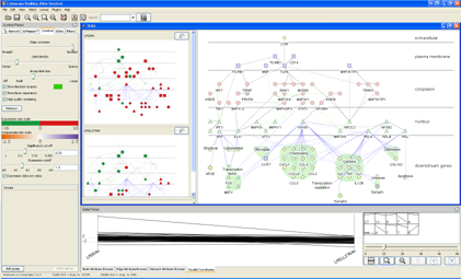
You will now have a view that should look something like the figure at right. The main network view still shows the complete TLR4 network with the original colouring. Two smaller views, one for each of the expression conditions we loaded, now appear to the left of these view. These are called the small multiple views and show the expression-based colouring for each condition. In the Parallel Coordinates tab, a graph has appeared with our two conditions represented as vertical axes and lines drawn to show the expression profile across the conditions. At the right-hand side, several small thumbnails appear, each showing a different expression profile and a number - these are the clusters of similarly-profiled genes Cerebral has generated from the loaded expression data. In the next sections, we will explore each of these views and functions in turn.
Step 2: Expression-coloured mini-views of the data
2.0: Click on a mini-view (either its name or within the mini-network) to promote its colouring to the main network view. (NB: to return to the original colouring, click again in the mini-view.)
2.1: Try panning, zooming and selecting nodes in either the main view or a mini-view - you will notice the views are all linked, so zooming in on the main view has the same effect in the mini-views.
2.2: You can resize the mini-views by both dragging the divider between the mini-views and main view, and by using the slider at the bottom of the mini-view pane, which controls how many columns are used to display the mini-views (this is useful when you have 4+ conditions loaded and want to see all their mini-views at once).
2.3: You can re-order the mini-views by clicking a mini-view's title and dragging it to the desired position. You will also note this changes the order of the vertical axes in the Parallel Coordinates view, and of the clusters in the cluster viewer. You can also re-order mini-views by clicking a vertical axis in the Parallel Coordinates view and dragging it to the desired position.
2.4: You can control which nodes are coloured according to the degree of their fold-change and the associated p-value by using the two sliders in the Cerebral tab of the Control Panel. The Significance cut-off slider specifies a p-value threshold, above which a node will not be coloured. At the default value of 0.05, all nodes with a fold-change meeting our default expression cut-off of +/-1.5 are coloured. Note that with this sample data, if we move the slider to 0.001, or type that value into the box, no nodes will be coloured as none have a p-value that low. The Expression cut-off slider and text box work in the same way - you can set the fold-change above or below which nodes will be coloured in. NB: Ratio vs non-ratio data. In ratio data, an increase of 20% is written as 1.20 whereas in non-ratio data, it would be written as 0.2. Cerebral scans each condition and looks for data in the -1.0 to +1.0 range - if there are no expression data points in this range, ratio data is assumed and this box is checked by default. If data is found in that range, non-ratio data is assumed and the box is unchecked. Either behaviour can be overidden by the user.
2.5: You can also change the colouring used for the mini-view expression scale using the Expression colour scale editor. Click on the coloured bar to bring up the editor. Let us try a few different colouring schemes to get some experience with the colour editor - remember to click the Apply button after each change to have it take effect in the network views:
- Change to a yellow:blue scheme by clicking the yellow/blue bar (2nd from top in the gallery)
- Specify your own solid 2-colour scheme by first clicking the yellow -16 to 0 segment at the top of the editor, then clicking the yellow swatch that appears near the minimum/maximum specification. Select your desired colour from the palette and click OK to apply the change. Do the same thing, changing the blue segment to whatever colour you please.
- Go back to the green/red solid scheme (1st line in the gallery). Click the green-black gradient button (to the left of the green/red bar, bottom icon). This adds a green gradient to the end of the colour bar, which is initially set to the -32 to -16 range. Our expression values range between ~-5 and +12, so let's set the green gradient to cover the range from -12 to 0 but typing these values in the Minimum/Maximum boxes. Now, click the red gradient and perform the same set of actions, setting a gradient to range from 0 to 12. Look at the mini-view colouring. You may have noticed that most of the nodes are coloured faintly, with only one bright red node. This is the result of having an outlier in the expression values - one node whose fold-change is much, much higher or lower than other nodes. The next colouring scheme will show you how to work around these outliers.
- Open the colour editor again and select the scheme with a small dark green section, a small light green section, a large yellow section, and small orangeish and red sections. Set the minimum value for the dark green bar to -5 and the maximum value for the dark red bar to 12. This provides a much more informative colouring, where the presence of a single outlier does not affect the degree of colouring of other interesting nodes.
Step 3: Profile view of the data
3.0: In the Parallel Coordinates tab of the Data Panel, two vertical axes appear, one for each experimental condition. Click on a vertical axis and drag it to re-order the conditions. Click the icon with three vertical lines to space the axes evenly.
3.1: You can pan and zoom in the Parallel Coordinates window just as you do in the main Cytoscape windows - right-clicking and moving the mouse up or down zooms in and out, which middle-clicking and dragging pans. The magnifying glass icons can be used to zoom into a selected region or zoom out.
3.2: Click your mouse near one of the vertical axes and, while holding down the mouse button, drag the mouse to create a rectangle on the vertical axis. A purple bar will appear, as will fold-change values. You can use this tool to select a fold-change range (try selecting from ~12 down to about 1 on the LPS04h condition). If you then click the funnel icon underneath the cluster diagrams, all the lines (nodes) that pass through the selected range will be filtered out (displayed as light grey lines in the Parallel Coordinates tab and their nodes will appear transparent in the main and mini-views). To un-filter the lines, click the icon of the funnel with the X.
Step 4: Comparison view of the data
4.0: The main view can be coloured to show the difference in expression values between two selected conditions. Click the comparison button for the LPS04h condition (the button with two small window icons to the right of the mini-view title, then click the comparison buttom for the LPSLL3704h condition (you can also shift-click the two conditions of interest to compare them). This tells Cerebral to colour the main view according to the change from the first selected condition to the second condition, and the main view's title will reflect this.
4.1: The difference colouring is a direct subtraction - the fold-change in condition 2 minus the fold-change in condition 1. A node's colour is determined by the magnitude of this difference. Clicking on the Comparison colour scale bar brings up the colour editor and allows you change the default colouring scheme.
Step 5: Clustering the data
5.0: At the right-hand side of the Parallel Coordinates tab, several small thumbnails are visible. These are clustered gene expression profiles - genes whose expression shows similar behaviour across different conditions. The clusters are calculated using the k-means clustering algorithm, with a default k of 10 (meaning 10 clusters will be created). An average expression profile representative of each cluster is shown in each thumbnail, along with the number of genes in the network that belong to the cluster.
5.1: Drag the slider to the left or right to change the k-value and, therfore, the number of clusters created. Smaller k-values mean fewer clusters and more variable profiles within a cluster. The best number of clusters for a given set can be difficult to determine, but we recommend trying values in the 10-20 range and evaluating the results by looking at the thumbnails.
5.2: Clicking on a cluster of interest filters out all other nodes - just the cluster members will be coloured in the main and mini-views, and only the members' lines will appear in black in the Parallel Coordinates viewer. Shift-clicking allows you to select multiple clusters simulatenously, while clicking anywhere in the network views or profile views will de-select clusters.