Cerebral Users' Manual
- 1. Overview
- 2. Installation
- 3. The display
- 4. Create Cerebral view dialog
- 5. Cerebral display options
- 6. Navigation
- 7. Groups
- 8. Saving and restoring a session
- 9. Overlaying data from multiple experiments
- 10. Hand placed layout
1. Overview
Cerebral (Cell Region-Based Rendering And Layout) is a Java plugin for the widely used open-source Cytoscape molecular interaction viewer. Given an interaction network and subcellular localization annotation, Cerebral automatically generates a view of the network in the style of traditional pathway diagrams, providing an intuitive interface for the exploration of a biological pathway or system. The molecules are separated into layers according to their subcellular localization. Potential products or outcomes of the pathway can be shown at the bottom of the view, clustered according to any molecular attribute data - protein function, - for example. Small multiple views enable a user to see expression data from 2 or more conditions overlaid on a network, while a difference view allows two conditions to be selected and a new view is coloured based on the changes between the selected conditions. An interactive k-means clustering tool also allows users to cluster their data, using a slider to adjust the number of desired clusters, and quickly select nodes based on cluster membership. Cerebral scales well to networks containing thousands of nodes.
2. Installation
Before installing the Cerebral plugin, you must have Cytoscape installed on your computer. You can download the latest version of Cytoscape from the Cytoscape.org downloads page.
Download both the latest version of cerebral.jar and prefuse.jar from the Cerebral Downloads page and save them in the Cytoscape plugins directory. This can be found at Cytoscape_X.x.x/plugins in whichever directory your applications/program files are stored.
Launch Cytoscape. If the Cerebral installation was successful, you will see a tab marked Cerebral in the Control Panel (CytoPanel 1 in Cytoscape 2.4 and earlier), and you will see two menu items - Create Cerebral View and Export Cerebral View in the Plugins menu bar. If you do not see the tab or the menu items, Cerebral has not been installed properly. Ensure the files were placed in the correct directory, and that you are launching Cytoscape correctly (launching it a certain way on some systems may not include all plugins during the load -if using Windows, load it using the .bat file).
Note that when you install an updated version of Cytoscape, you will have to move Cerebral.jar and prefuse.jar to the new plugins directory.
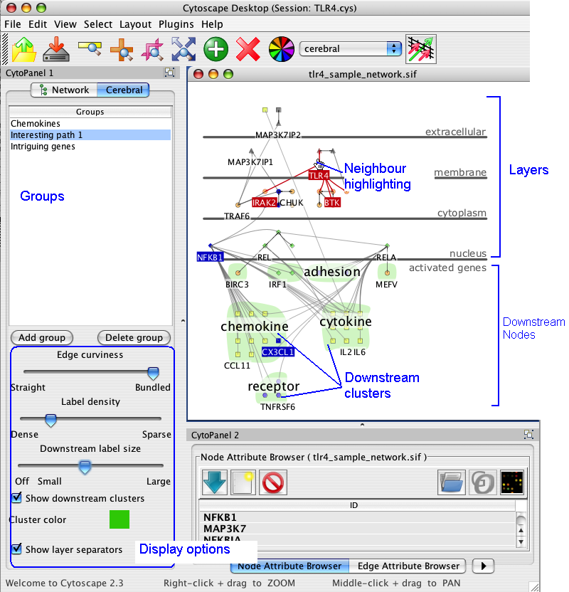
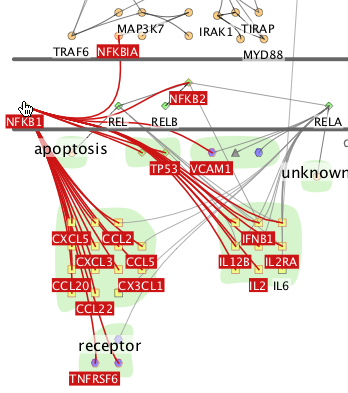
3. The Display
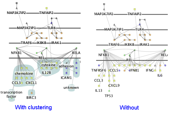
Cerebral creates views of the network in the style of traditional pathway diagrams. Cerebral uses a node attribute, such as localization, to restrict the placement of nodes into specific layers. The products/outcomes of a pathway can easily be positioned in the downstream nodes layer at the bottom without changing localization annotation. The nodes in the downstream layer can be clustered into groups. Cerebral visually highlights neighbours and clusters.
4. The Create Cerebral view dialog
Choosing Plugins->Create Cerebral View brings up the following dialog.
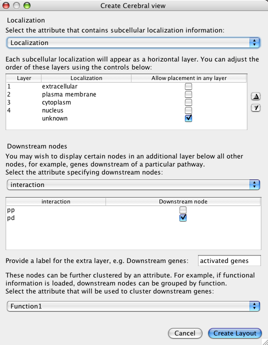
The dialog has two major sections that will be described below:
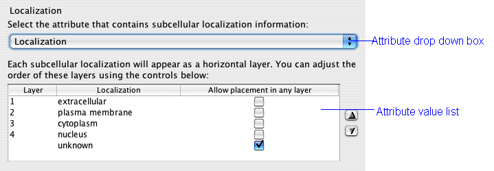
The localization attribute has the greatest effect on the appearance of your network. This setting defines the major layers that restrict the placement of nodes. The drop down box is populated with all of the node attributes associated with your network. You can load additional node attributes by first closing the dialog and then choosing File->Import->Node attributes... from the Cytoscape menu.
The list below the drop down box fills with the unique node values for the chosen attributes. The order of the values in the list is the order in which the layers will appear in your network. Change this order by first clicking an value to select it and then using the up and down arrows to the right if the box.
If you click the Allow placement in any layer box, then proteins with that attribute will not be restricted to a layer band. They will appear in one of the other layers near to their interacting neighbours. This is particularly useful for nodes that do not have localization information. It is advisable to visually distinguish these nodes with the VizMapper to distinguish them for actual members of a layer.
Currently it is not easy to merge multiple attributes into a single layer. Suppose for example you had some nodes marked as cytosol and some nodes marked as cytoplasm and you wished to have them displayed in the same layer. You must edit the node attributes file by hand and change every instance of cytosol or cytoplasm to cytosol/cytoplasm. When you reload the node attributes file, the list will show a single layer named cytosol/cytoplasm.
Some proteins have multiple locations within the cell. We offer the following suggestions for handling this type of data
1. Label all dual location proteins in a consistent way within your localization node attributes file. For example, assign proteins that are located in both the cytoplasm and the nucleus the attribute cytoplasm/nucleus. Then sort the layers as cytoplasm, cytoplasm/nucleus, nucleus when you create the layout. An additional band with these dual location proteins will appear in your diagram.
or
2. Check the Allow placement in any layer box for all multiple location proteins. These proteins may appear in any layer, but will likely appear in layers near to their interacting neighbours. You can then visually highlight them by assigning them a colour with VizMapper (instructions in the Cytoscape manual)
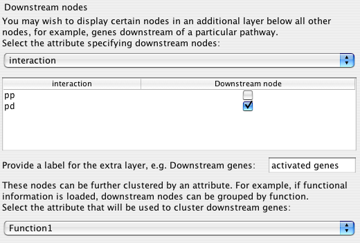
Many traditional pathway diagrams list genes regulated by a pathway at the bottom of the diagram. Cerebral offers a way to mimic this behaviour without changing your node attribute files. Cerebral will move nodes to the bottom of the pathway that satisfy the criteria specified in this step.
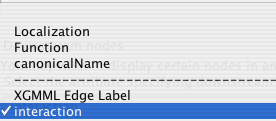
The drop down box shows all of the node attributes and edge attributes associated with the network. The node attributes appear above the dashed line and the edge attributes below.
After choosing the attribute category, the list below the drop down box fills with the unique values. Click the Downstream nodes box to have all nodes with the matching value positioned at the bottom of the diagram.
If you select an edge attribute, it is the target of the edge that is affected. The target is the node to the right of the attribute in your Cytoscape files. For example, if your .sif file had the following lines
NFKB1 activation CCR7
REL activation IFNB1
and you chose the interaction edge attribute and activation, then CCR7 and IFNB1 would be placed at the bottom of the diagram. NFKB1 and REL would be unaffected.
Finally type in a label for the extra layer
![]()
When Cerebral draws the network, it places nodes at locations that make the interactions between nodes as clear as possible. For the downstream nodes, it may be preferable to emphasize the functional role of the nodes. Choosing a node attribute in this final drop down box will cluster the downstream nodes into groups that share the same attribute values.
5. Cerebral display options
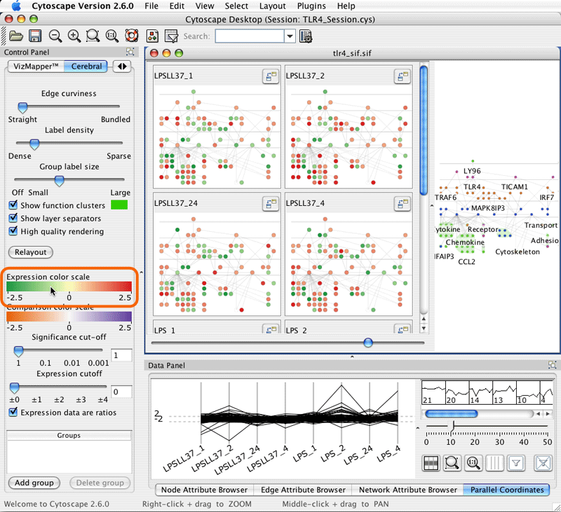
Cerebral has many options to customize the appearance of the display. Access them by clicking on the Cerebral tab in CytoPanel 1, located on the left side of the screen.
Note: Due to a bug in Cytoscape, the Cerebral panel might not appear when you click on the tab. To work around this bug, click the tabs in order from left to right until the Cerebral panel appears.
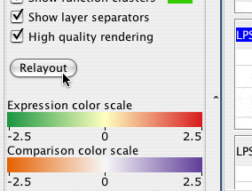
The display options appear in the lower half of the Cerebral panel. The groups functions are described in section 7.
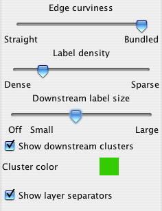
Some proteins may have several interactions. To simplify the appearance of the diagram, Cerebral ties the edges leaving these proteins into bundles. You can control how tightly these edges are bound with the Edge curviness slider.
Cerebral displays readable non-overlapping labels at all zoom levels. The size, font, and text of the labels are controlled through VizMapper. The Label density slider controls how many labels Cerebral attempts to fit onto the screen.
5.3 Downstream layer appearance
If you specified a clustering attribute when you created your display, Cerebral will write the attribute value above the cluster. You can use the Downstream label size slider to control the size of this label or turn downstream labeling off completely.
Cerebral will show a coloured blob around all nodes in a cluster. You can choose this colour by clicking on the colour swatch beside Cluster color or turn it off completely by unchecking Show downstream clusters.
You can turn off the layer separators by unchecking Show layer separators. Currently the only way to change the text of the layer separators is by changing the localization attribute values in your node attributes file.
6. Navigation
Pan the display by pressing the middle mouse button and dragging the
mouse in any direction.
Zoom in by pressing the right mouse button and moving the mouse up.
Zoom out by pressing the right mouse button and moving the mouse down.
As you freely move the mouse around the screen, passing over a node
will immediately highlight it in red, along with all of its direct
neighbours.
Selected nodes are highlighted in blue. You can select nodes in several ways:
- Left-click and drag a rectangle around the nodes of interest
- Left-click on a single node
- Left-double-click on the background of a downstream group to select all the nodes in the group
- Use the Cytoscape filters function to select nodes
In all these cases, you can select multiple nodes by holding down the shift key when you click.
7. Groups
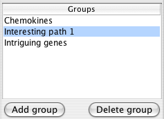
Groups allow you to form collections of nodes while exploring your network. These groups are visible in the rest of Cytoscape as the attribute Cerebral groups with the group names as values. You can change the visual appearance of group members by selecting that attribute in VizMapper.
The list of groups appears in the top half of the Cerebral panel. Clicking on a group name in that list selects all members of the group highlighting them in blue.
Groups can be renamed by double-clicking on their name.
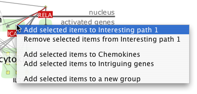
Right-clicking on a node in the display brings up a popup menu allowing you to add the node to any group, or delete it from the current group. If you have selected multiple nodes, all of them are added or deleted from the group.
8. Saving and restoring a session
To save your Cerebral view between Cytoscape sessions, save it as a Cytoscape session (.cys) file by selecting File->Save. Restore the session by selecting File->Open.
If you close a Cerebral view within a session by closing the window or right-clicking the network and selecting Destroy view you can restore it by choosing Plugins->Restore previous Cerebral views. Note that right clicking a network and choosing Create view will open a regular view of the network without Cerebral's extra features.
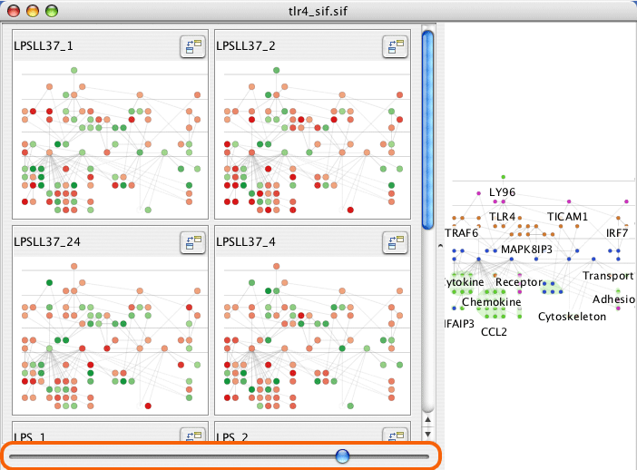
9. Overlaying data
Cerebral 2.0 displays data from multiple experimental conditions simultaneously. Each condition colour codes a small multiple view of the data. This section will show you how to load data, reorder, filter, and compare conditions.
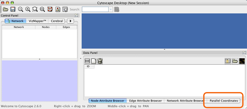
First load all of your experiment data into node attributes using Cytoscape's standard data loading features. e.g. File->Import->Attribute from Table (Text/MS Excel)... Next click on the Parallel Coordinates tab in the data panel.
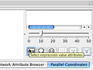
Click the "Select expression value attributes" button.
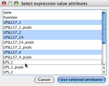
Choose all the node attributes that contain experimental data. Select multiple attributes by holding down the Ctrl key. If you have associated p values, do not select them here (see filtering with p-vals )
Each attribute will create a mini graph view of the data.
A graph is created for each chosen experimental condition. The graph is colour coded according to the experimental values. You can zoom, pan, and select in any of the graph displays and the effect is linked across all displays.
9.2.1 Resizing/reordering displays
Drag the divider between the main and mini-view graphs to resize the displays.
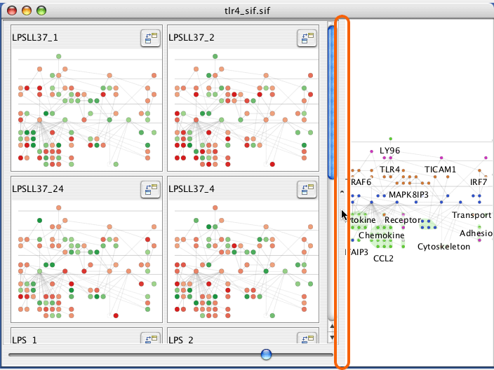
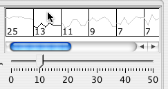
The slider at the bottom of the mini-graphs sets the number of columns for the mini-graphs.
Click and drag on the title of a mini-graph window to reorder, or use the axes in the parallel coordinates view.
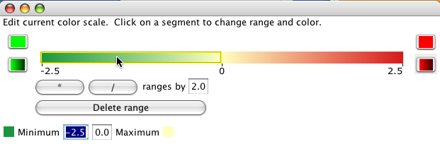
The colours for each mini-graph display are assigned using the data associated with that graph's node attribute and the Expression colour scale. Clicking the title of a mini-graph display will colour the main display according to the mini-graphs data values. Click on the Expression colour scale bar to bring up the colour editor.
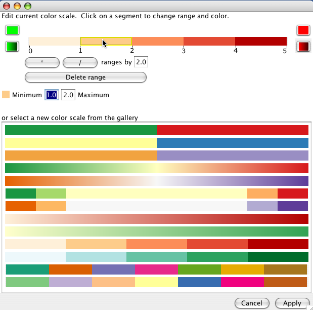
The colour scale assigns a value range to a colour. The gallery provides some useful default colour scales, though the exact ranges will likely need to be edited. You can change the size of all the ranges by using the * or / buttons. Alternately, click on a single range to edit the minimum and maximum value for the range.
Solid ranges use the same colour for values within a range.
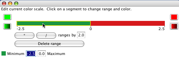
Gradient ranges linearly interpolate the colour from the minimum value in the range to the maximum value.
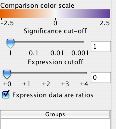
9.4 Significance and expression filtering
The Cerebral panel has two filters that apply across all experimental conditions. The expression filter operates directly on the values data values associated with each node attribute. All nodes whose values do not exceed the expression filter are drawn transparently.
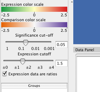
The significance filter uses a significance value associated with each experiment value. Cerbral searches for a node attribute named either "pvals, _pvals, sig, or _sig". For example, if your experiment data was in node attributes names "Time01H" and "Time02H", your significance values should be in attributes named "Time01H_pvals" and "Time02H_pvals". If the significance value associated with a node is not below the signficane cutoff, then the node is drawn transparently."
The main Cerebral view can show the direct computed difference between two conditions. Click the "Compare against another condition button" and then click the title of another experimental condtion. The main display shows the computed difference using the Comparison colour scale as Dx = Bx - Ax. If the value did not pass the significance filter in either A or B, then the value of 1.0 is used.
You can alternately choose conditions for comparison by clicking the label for condition A and then shift+clicking the label for condition B in either the mini-graph or the parallel coordinates views.
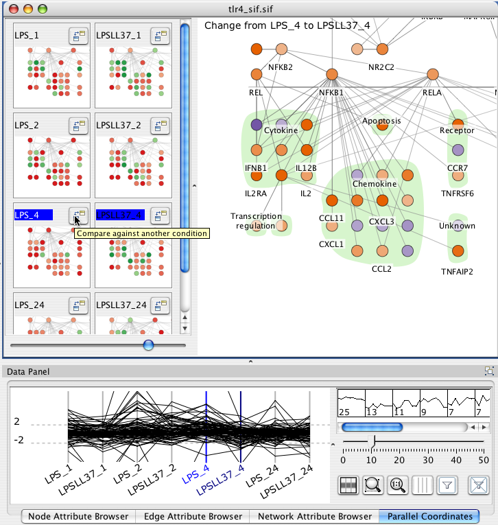
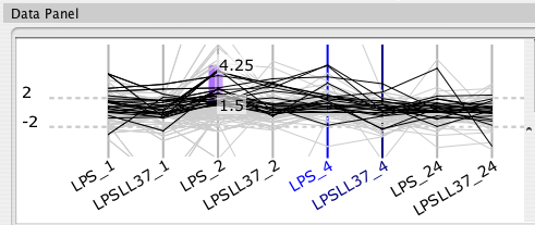
Each selected node attribute appears as an axis in the parallel coordinates display. Each line in the display represents a node. The line crosses each axis at the value for the given node attribute. You can reorder axes by clicking and dragging them. Dragging a rectangle around an axis defines a filter range. A line must pass through the filters on all axes to be selected.
You can pan and zoom the parallel coordinates display just like the main display using the right and middle mouse buttons
The right side of the paralle coordinates panel shows the data values clustered with k-clustering. Choose the k value by dragging the slider. Then click on the representative cluster shape to select all nodes belonging to the cluster
For some data sets, an increase of 20% is represented as 0.20, whereas for ratio data sets it is represented as 1.20. Cerebral attempts to automatically detect ratio data by checking if there are no data points between -1.0 and 1.0. Use the "Expression data are ratios" check box to override the default behaviour. The Parallel Coordinates display will exclude the range -1.0 to 1.0 when this box is checked.
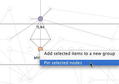
10. Hand placed layout
You can position key nodes by hand, pin them in place, and then have Cerebral automatically choose locations for the remaining nodes. Right click on important nodes and select "Pin node" from the menu. Then click the "Relayout" button in the Cerebral panel. Cerebral will select new locations for all the unpinned nodes. The nodes remained pinned, until you right click them and select "Unpin node".